60th Annual Report on Research 2015

Project Objectives:

Advances in shale gas technology, and in particular hydraulic fracturing, have enhanced production from unconventional reservoirs [Drake, 2007; King, 2010; Boyer, 2006; Bowker, 2007]. Characterization and imaging of hydraulic fracturing systems, however, has proven to be a challenging problem, primarily due to complexity of fractured systems and limited observations that can be used to infer the properties of matrix and fractures. This project, which constitutes a new research direction for the Principle Investigator, aims at characterizing fractures by developing computational inverse methods for combining monitoring data with mathematical models of the underlying multiphysics processes. This report summarizes the progress made by the PI on developing a data assimilation framework for characterizing the geometric and hydraulic behavior of planar fractures and complex fracture networks. As a new direction grant, this project has enabled the PI to extend his inverse modeling research to characterization of hydraulic fracture properties and enable him to continue to work in this area by seeking additional research funding.

Fracture Models:

We have considered the characterization of both planar fractures and complex fracture networks from flow-related data. In this report, we discuss these two fractured systems separately.

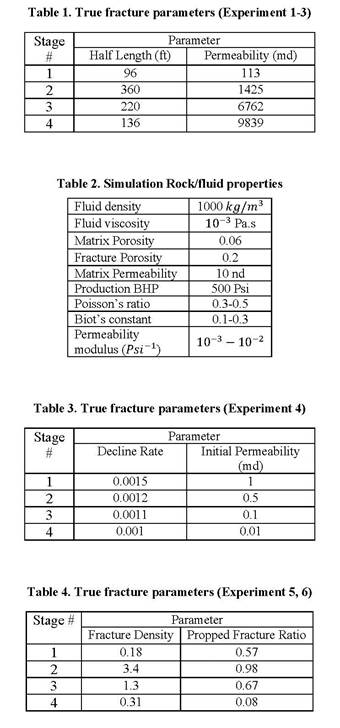
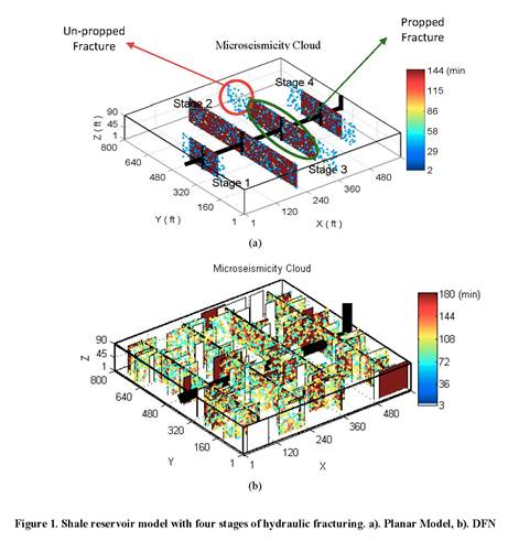
Planar Fractures are modeled as rectangles (Figure 1a) with their length and hydraulic conductivity as parameters. Tables 1 and 2 provide a summary of fracture parameters and reservoir properties for the reference model used in our example. Since, the permeability of rock changes during the production [Clarkson, 2012], we also use the correlation proposed by Bachman [2011]

(1)

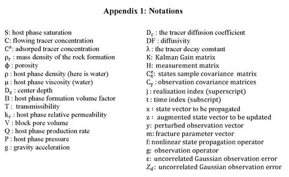
to include this effect (see Appendix 1 for notations). Discrete Fracture Networks are modeled using a network consisting of small fractures that populate the reservoir. A stochastic model with a control parameter, called the fracture density, is used to model the number of fractures per unit volume of the formation [Caca et al 1990]. Figure 1b illustrates a fracture network generated by this stochastic model. In this case, the objective is to estimate fracture density in the reservoir.

Fracture Characterization Method:

We have adapted the EnKF data assimilation approach [Evensen, 2007] for assimilation of monitoring and production data. The EnKF consists of a forecast step to predict the measured data using an appropriate model of the process, followed by an update step that integrates the predictions from the forecast step with observed data to improve the fracture parameters.

 

Forecast Step is represented by the governing flow and transport equations. The governing equations for a single phase transport system is given by Eqs. 2 and 3 (solved using [Eclipse 2011])

 

(2)

(3)

The goal of the forward model is to establish a relation between model parameters (fractures properties) and the observed monitoring data (through predictive analytics). The Update Step is an ensemble form of the Kalman filter [Kalman, 1960] that was propose by [Evensen, 2007]. The forecast and update steps of the EnKF can be summarized as a state space model of the form:

     ,    (4)

 ,     (5)

In this project, we implemented an adaptive localization method named hierarchical EnKF, which was introduced by Anderson [2007] to alleviate the impact of the spurious updates.

Numerical Experiments and Discussion:

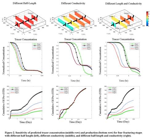
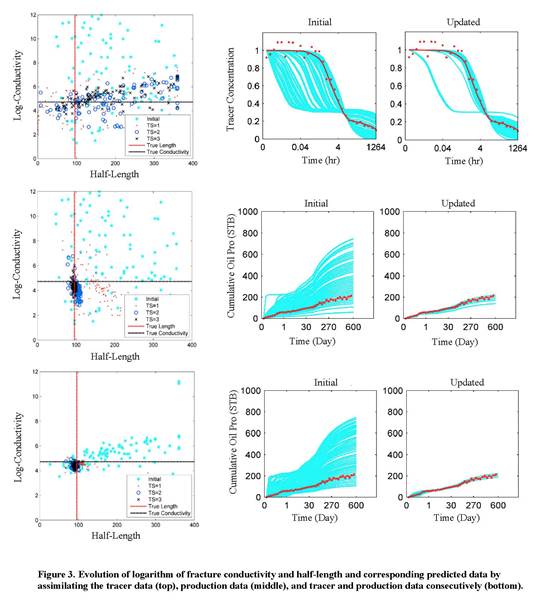
Experiment 1: Planar Fractures. Figure 2 displays the sensitivity of the predicted tracer concentration and production to fracture model parameters (fracture length and conductivity), for four fracturing stages. The production predictions appear to be more sensitive to fracture length while tracer concentration tends to be more sensitive to fracture conductivity. Figure 3 summarizes the estimation results using the tracer (First row), production (Second row), and tracer followed by production (Third row) data. The first column of Figure 3 shows the cross-plot of fracture half-length (x-axis) and fracture conductivity (y-axis), the two unknown parameters of the planar model, for Stage 1 of the treatment. The intersection of the two axes represents the reference values for each parameter. The values before data assimilation, shown in cyan, are scattered around the two axes and show significant uncertainty. The final ensemble is more concentrated around the intersection point (where reference fracture permeability and half-length values are located). The corresponding predicted tracer concentration profiles or production data for the initial (Middle column) and final (Right column) ensembles are also shown in Figure 3. The initial uncertainty in fracture parameters is clearly reduced. In addition, the results show that the tracer data is not as sensitive as production data is to fracture length.

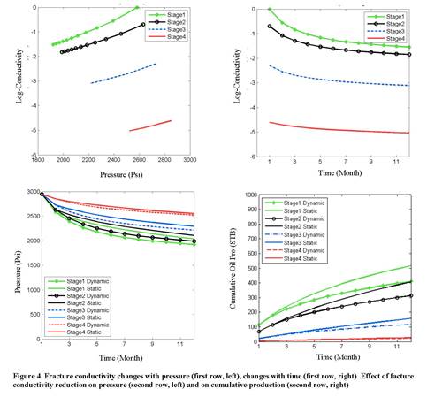
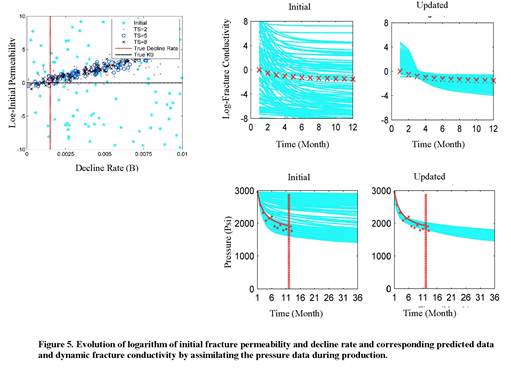
Experiment 2: Dynamic Planar Fractures. Using Eq. 1, the changes in fracture conductivity and production as a function of pressure and time are shown in Figure 4. The results of estimating initial fracture permeability and conductivity decline rate from pressure data for Stage 1 are depicted in Figure 5. The initial values for these parameters are scattered around the two axes and show significant uncertainty. The final values are concentrated around the intersection, which corresponds to the reference fracture permeability and decline rate. The estimated fracture conductivity and pressure data for initial and final ensemble show reduction in uncertainty mainly in conductivity.

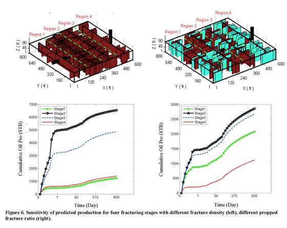
Experiment 3: Stochastic Fracture Networks. We have also performed experiments for estimation of fracture parameters using the fracture network model. Figure 6 shows the sensitivity of cumulative production trend to open fracture density. The estimation results for fracture density and propped fracture ratio in Stage 1 are shown in the First and Second rows of Figure 7, respectively. The EnKF is then used to update these two parameters based on available production data. For different time steps, the mean and variance of the updated parameters are shown with cyan color while the reference parameters are indicated with red crosses. It can be seen that the updated ensemble is closer to the reference fracture parameters and have smaller variance. The corresponding predicted production based on the initial and final ensemble of parameters confirms this result, showing significant reduction in the initial uncertainty.

Ongoing and Future Work:

Our ongoing work is to incorporate the spatial heterogeneity in fracture parameters for a more realistic representation of fracture networks.