Reports: UR955347-UR9: Computational Studies of Osmotic Membranes for Petroleum Wastewater Reclamation
 printer friendly
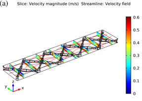
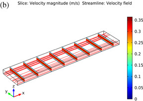
Fig.
1. Contours
of velocity magnitude on eight yz-slices and streamlines in (a) spacer-filled
channel and (b) unobstructed channel.
Fig.
2. Streamlines
(v, w) on three yz-slices in spacer-filled channel. The slices are cut
In
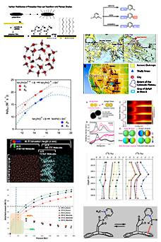
industrial BWRO operation, the average longitudinal velocity of the retentate
stream gradually reduces as it travels along the pressure vessel due to water
recovery. To develop a system level model for pressure drop, a parametric
analysis is carried out by varying velocity at the inlet of the computational
domain. The pressure differential is recorded and compared with correlations of
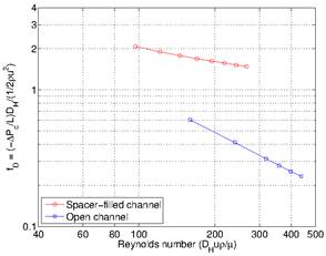
channel flow. The Darcy friction coefficient is calculated as follows:
(1) In the flat narrow channel the 3D numerical simulation matches
closely with the theoretically derived relationship fD=96/Re.
However, in the spacer-filled channel, fD is several times larger if
the Reynolds number is the same.
Fig. 4. Darcy friction coefficient vs Reynolds number.
.
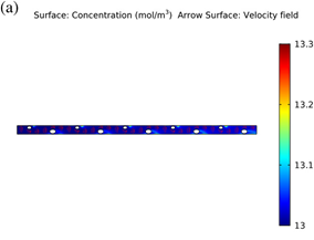
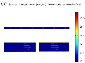
It is found that in the spacer-filled channel Salt concentrations and flow arrows are plotted on an
xz plane for both the spacer-filled and unobstructed channels, as shown in Fig.
5(a). It is observed that concentrated islands
are isolated in zones near the spacer filaments, where the flow is stagnant.
These are areas associated with smaller fluxes. The concentrated region is
thinner in regions with high fluid velocities. The concentration polarization
profile in spacer-filled channel differs from the one in the empty channel,
where a concentrated layer gradually develops along the channel severely
reducing permeation flux. Fig. 5. Salt
concentration with fluid flow arrows on xz plane of (a) spacer-filled channel
and (b) unobstructed channel.
The mass transfer coefficient km is related
to salt concentration gradient at the membrane wall by the following equation:
(2) Using the concentration gradients reported by the
converged CFD solution and Eq. 2, the local mass transfer coefficients in the
computational domain based on four different values of inlet velocities are
calculated. This is because as water permeates through the membrane, the
average longitudinal velocity decreases in a long pressure vessel, leading to a
reduction in km. It is seen that km reduces with respect
to both location and longitudinal velocity in open channel. For the
spacer-filled channel, km reduces mostly with respect to
longitudinal velocity. However, at a given velocity, it appears that km
profile is repeated from cell to cell and there is no significant decay in
cell-average km with respect to location.
The cell-average km over the
length of five unit cells is calculated and it plotted as a function of
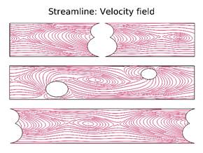
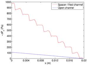
Fig.
3. Pressure
differential along feed direction with average feed velocity of 0.25 m/s. The
x-axis is a horizontal line cut at y = 1/4 width and z = 1/2 of the
computational domain.
![]()
![]() , or
, or ![]() .
.
![]()
![]() on
a loglog scale, as showed in Fig. 6. Both follow straight lines, however, the
slopes and magnitudes are different. In the open channel,
on
a loglog scale, as showed in Fig. 6. Both follow straight lines, however, the
slopes and magnitudes are different. In the open channel, ![]() ;
the power law index is very close to 1/3 as indicated by the boundary layer
theory. In the spacer-filled channel,
;
the power law index is very close to 1/3 as indicated by the boundary layer
theory. In the spacer-filled channel, ![]() .
The existence of spacer filaments significantly enhances mass transfer.
.
The existence of spacer filaments significantly enhances mass transfer.
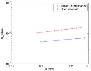
Fig. 6. Cell-average km as a function of average feed
velocity.