58th Annual Report on Research 2013 Under Sponsorship of the ACS Petroleum Research Fund

During the first year of our research a new code was developed and it was validated. The compressible form of the conservation equations for mass, momentum, energy, and conserved scalar are solved. The computational domain is discretized on uniform finite-difference gird points. The flow solver is fourth-order accurate in space and second order accurate in time. The scheme is the predictor-corrector scheme of MacCormack modified by Gottlieb and Turkel. A parallel version of the code is developed using Message Passing Interface (MPI) subroutines for data communication between processors. The parallel code is scalable for simulations with grid points in the order of several billions.

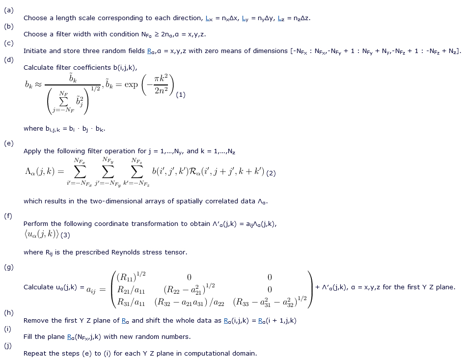
An initial condition code is developed to produce velocity perturbations based on a digital filter method. [1] This method generates fluctuations based on prescribed length scales and Reynolds stress tensor satisfying a locally given autocorrelation function. This code is capable of generating fluctuating velocities for turbulent free shear layers, i.e. mixing layer and jet, and for both spatial and temporal simulations. The algorithm for generating velocity fluctuations used in the initial condition code is summarized below:

In order to validate the flow solver, governing equations are solved for the temporally evolving turbulent mixing layer with convective Mach number of 0.2. Computational domain lengths in x, y and z directions are 300d_θ0, 150d_θ0 and 100d_θ0 with grid points 1260, 631 and 421 respectively, where d_θ0 is initial momentum thickness. Periodic boundary conditions are imposed in homogeneous directions (x and z), while in transverse direction (y) the boundary conditions are characteristic slip walls at which normal component of velocity is zero at all times. The mean flow is initialized with hyperbolic tangent profile in streamwise direction, while the mean vertical and spanwise velocities are zero. The pressure, temperature, and density fields are initially uniform and the conserved scalar is initialized with hyperbolic tangent profile such that its values in upper and lower streams are 1 and 0 respectively. To initiate turbulence, three dimensional perturbations generated by the initial condition code are imposed on mean velocities. It is observed that after a transitional period, flow reaches a self-similar state in which the shear layer growth rate, = (dd_θ∕dt), approaches a constant, and turbulent statistics are collapsed across self-similar coordinates. Self-similar state starts at t = 250 and it continues until the end of the simulation at t = 600.

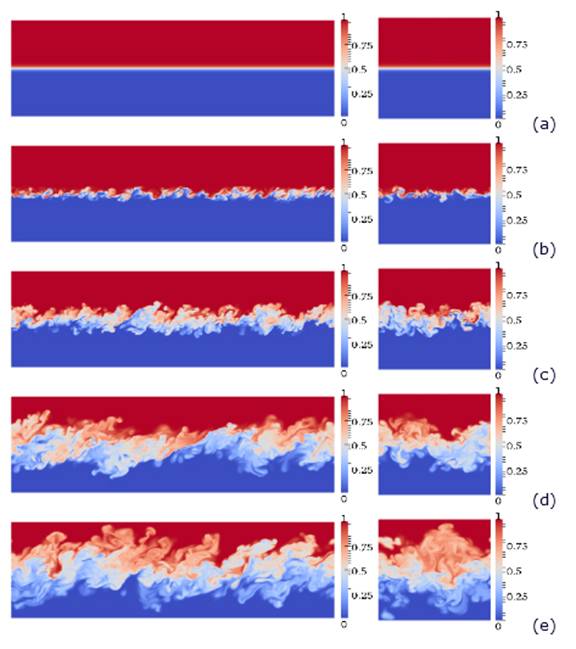
Figure 1: Time evolution of the conserved scalar in the mixing layer, (a)t = 0, (b)t = 20, (c)t = 100, (d)t = 400, (e)t = 600. Figures on the left represent XY , and on the right Y Z planes.

Figure 1 represents the instantaneous contours of the conserved scalar showing evolution of the mixing layer from initial time to end of the simulation in XY and Y Z planes located in the center of the computational box. It is observed that using initial conditions based on the digital filter method leads to a smaller transitional time compared to the same simulation with initial perturbations from linear stability theorem. It can be seen that in early times (Fig. 1.b), rollers and braids are formed and the pairing of the rollers occurs at later times.

The growth rate of mixing layer is 0.0135, which is close to 0.014 reported in literature for incompressible mixing layer. In Fig. 2, the time averaged streamwise velocity, and components of the normalized Reynolds stress are compared with other studies. [2, 3, 4] It can be seen that the shape of the profiles and the peak values of Reynolds stresses are in good agreement with previous results.

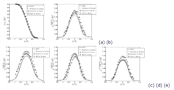
Figure 2: Comparison of (a) normalized streamwise mean velocity and (b)-(e) normalized components of Reynolds stresses with numerical and experimental data.

References

[1]   M. Klein, A. Sadiki, and J. Janicka. A digital filter based generation of inflow data for spatially developing direct numerical or large eddy simulations. J. Comput. Phys., 186(2):652–665, April 2003.

[2]   BW Spencer and BG Jones. Statistical investigation of pressure and velocity fields in the turbulent two-stream mixing layer. AIAA Paper 71-613, 1971.

[3]   James H. Bell and Rabindra D. Mehta. Development of a two-stream mixing layer from tripped and untripped boundary layers. AIAA Journal, 28(12):2034–2042, December 1990.

[4]   C. Pantano and S. Sarkar. A study of compressibility effects in the high-speed turbulent shear layer using direct simulation. J. Fluid Mech., 451:329–371, February 2002.