58th Annual Report on Research 2013 Under Sponsorship of the ACS Petroleum Research Fund

We have finished the prediction of microseismic event locations, velocity inversion, and the integration of microseismic and welltest data in heterogeneous case in this one-year period. To estimate the microseismic event locations, the real velocity model and ensemble velocity by EnKF  are used here, respectively.   

Part 1: The estimation of microseismic event locations

The event location results are obtained using EnKF by adding one monitor well one at a time. The number of ensemble members is 30. By assimilating the first arrival times from one monitor well, the estimated fracture width and height obtained using EnKF do not match the real value very well. However, the results using EnKF are significantly improved through using four monitor wells as shown from Figure 1. The estimated fracture width and height obtained using EnKF look reasonable. The real velocity structure is used in the above cases. We further study the uncertainty for the prediction of microseismic by the ensemble of the velocity. The estimated z-coordinate is biased from true when using the incorrect velocity structure with a large mean absolute error (E = 32.3), and is improved by using an ensemble of velocity structures which considers the uncertainty in velocity. The mean absolute error is reduced to 21.0 (Figure 2). Among these three scenarios, estimates obtained using the correct velocity structure is the best of all with the smallest mean absolute error of 15.2.

Part 2: The integration of microseismic and welltest data

We consider a synthetic two-layer heterogeneous example. As shown in Figure 3, we have 20 by 20 by 2 grid system with grid size of 200 ft by 200 ft by 50 ft. The active well is in the middle of the reservoir at grid (10, 10) and perforated in both layers. Cap rock is on top of the reservoir layers and its velocity is assumed known. Four monitor wells that are located at the corner gridblocks (2, 2), (2, 19), (19, 2) and (19, 19). Each monitor well has 11 microseismic receivers above the reservoir and 20 ft apart from each other with the first receiver right on the top of the reservoir. The model for calculating the first arrival time is 400 by 400 by 40 3-D grid with 5 ft by 5 ft by 5 ft as the grid size.

Perforations are shot in the middle of both layers and the first arrival time data of P-wave and S-wave are recorded at receivers in the 4 monitor wells. The well is produced at 1500 STB/D liquid rate for 2 days and shut in for another 2 days. The pressure data are recorded during the 2-day drawdown and 2-day buildup at the active well and the four monitor wells. In the following cases, 4 by 11 first arrival time data of P-wave and S-wave, 10 pressure drawdown and 10 pressure buildup data (logarithmically spaced) at the active and monitor wells, and layer rate data are assimilated to update porosity and log-permeability fields. The results show that assimilating both microseismic and well test data provides better resolution than using only each of datasets. Figure 4, 5 shows the overall uncertainty reduction of porosities in two layers after assimilating both microseismic and well test data by plotting the standard deviation ratio of the final ensemble after assimilating both microseismic and well test to the prior standard deviation.

Part 3: Future work

We will focus on how we can provide best origin time information of microseismic events in the next research stage which will be an important supplementary to the previous research. The inversion of event location and velocity and the integration of microseismic and welltest data in heterogeneous case will be tested in the next year of this project.

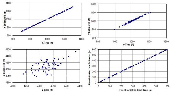
Figure 1: The cross-plot of the microseismic event location (x, y, z) and event occurrence time between the true and the estimated after assimilating first arrival times from all 4 monitor wells (EnKF)

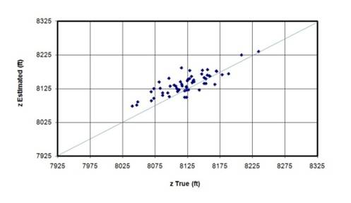
Figure 2: The cross-plot of z-coordinate between the true and the estimated using correct, incorrect and an ensemble of velocity (E=21.0)

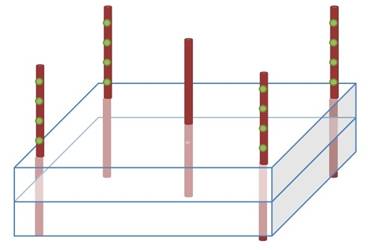
Figure 3: Reservoir and well schematic, two-layer heterogeneous example

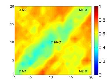
Figure 4: Posterior to prior STD ratio of porosity in first layer after assimilating both microseismic and pressure data  

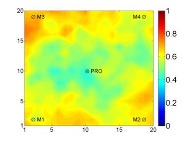
Figure 5: Posterior to prior STD ratio of porosity in second layer after assimilating both microseismic and pressure data